Abstract

This works deals with the processing and interpretation of GPR data which were collected during the first day of the practical field work of the training course of GPR applications for civil engineering, organized at the University of Malta, Valletta campus, in the frame work of COST Action TU1208.
The data were collected inside the Chapel of the Church of Jesuits located in Valletta campus, through the Stepped Frequency Continuous Wave Radar (SFCW), a prototype developed by Raffaele Persico and his team. The data collected in frequency domain, were transformed in time domain, and an interpretation of Data in 2D scans and 3D is shown. The procedure of processing follows some basic steps, such as moving starting time, gain, moving background, 1D filtering and migration. The main purpose of this study was the detection of buried structures under basement through the use of GPR.
Elaborated by
Authors: Hamza Reci1, Michal Dabrowski2, Giovanni Musolino3
1Institute of Geosciences, Energy, Water and Environment, Polytechnic University of Albania, e-mail: reci.jack@gmail.com
2 PhD student , Nicolaus Copernicus University in Torun, Faculty of Earth Science, Department of Geology and Hydrogeology, e-mail: mh.dabrowski@gmail.com
3 Freelance Civil Engineer – e-mail: musolino.giovanni@gmail.com
Introduction
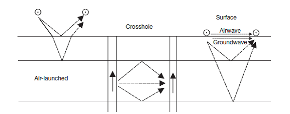
Ground-penetrating radar (GPR) enables the noninvasive characterization of the subsurface using electromagnetic (EM) waves. Early investigations include measurements of glacier, ice sheet, and permafrost. Nowadays, a multitude of applications exist for this high-resolution geophysical tool, which includes agricultural, archaeological, environmental, geotechnical, hydrologic, civil engineering and sedimentologic applications. Several books (Conyers and Goodman, 1997; Daniels, 2004; Jol, 2009, Benedetto and Pajewski, 2015), book chapters (Annan, 2005a,b; Blindow, 2006), and review papers (Annan, 2002; Huisman et al., 2003; Knight, 2001; Neal, 2004; Slob et al., 2010, Amir M. Alani et al., 2013) describe the principles of GPR technology, discuss the required processing steps, and show a multitude of existing and emerging applications. GPR measurements can be applied using different setups; air launched, crosshole, and surface-based (Figure 1). Here, the source and receiver antennae are indicated as solid arrows, which reflect the dipole nature and indicate that polarized electromagnetic fields are emitted and received respectively. Conventional processing and inversion methods for GPR data are often using ray-based methods originally developed for seismic data or using far-field high-frequency approximations. In several cases, this approach is sufficient, as long as the main focus is on the propagating nature of the waves. If the focus is on specific EM properties of a material that influence the wave dynamics, such as dipolar vectorial radiation patterns, polarization effects, or reflection coefficients, the scalar seismic techniques are no longer appropriate and specific EM processing and inversion techniques are necessary.
The Maxwell’s equations govern the EM wave propagation in a homogeneous space, a homogeneous half-space, and a horizontally layered earth, which are dependent on Relative permittivity εr, conductivity σ, and velocity v for selected materials (tab.1).
Table 1. Relative permittivity εr , conductivity σ , and velocity v for selected materials.
| Media | εr | σ(mS/m) | v(m/s) |
|---|---|---|---|
| Air | 1 | 0 | 0.3 |
| Distilled water | 80 | 0.01 | 0.03 |
| Fresh water | 80 | 0.5 | 0.03 |
| Seawater | 80 | 3000 | 0.01 |
| Dry sand | 3-5 | 0.01 | 0.13-0.17 |
| Saturated sand | 20-30 | 0.1-1 | 0.05-0.07 |
| Silt | 5-30 | 1-100 | 0.05-0.13 |
| Clay | 5-40 | 2-100 | 0.05-0.13 |
| Limestone | 4-8 | 0.5-2 | 0.11-0.15 |
| Granite | 6 | 0.01-1 | 0.12 |
| Dry salt | 6 | 0.001-0.1 | 0.12 |
| Ice | 3 | 0.01 | 0.17 |
The data were collected inside the Chapel of the Church of Jesuits located in Valletta campus, through the Stepped Frequency Continuous Wave Radar (SFCW), a prototype developed by Raffaele Persico and his team (Giovanni et al., 2002). The Jesuits' church is one of the oldest churches in Valletta, Malta, and one of the largest in the diocese. The site, comprising a college and a church is bounded by four streets occupying the whole area, as soon as Valletta was built, the Jesuits expressed an interest in building their own College there, since the city was considered the furthest bastion of Christianity against the Ottoman threat. The Church of the Jesuits was originally the church of the college, back at the end of the 16th century. But there are downsides to residency in a fortified city: on 12th September 1634 a violent explosion in the Order’s gun-powder magazine claimed many victims, along with severe damage to the surrounding area, including the church. In 1635 the Tuscan architect Francesco Buonamici undertook the restoration of the church, giving it the monumental baroque facade and imposing internal dome that we can admire today.
In 1662 the wealthy Maltese goldsmith Pietro Rosselli purchased the second chapel on the left in the church and appointed Mattia Preti to paint a triptych celebrating the life of St Peter. Preti was still a newcomer to the island and took this opportunity to produce three of his best works, in themselves good reasons to visit the church. He painted the two big lunettes with the Saints Peter and Paul led to martyrdom and the Martyrdom of St Peter, and the altar-piece depicting the Liberation of Saint Peter. According to the Acts of the Apostles Peter was rescued from imprisonment by an angel who put the jailers to sleep and caused Peter’s chains to fall away. Mattia Preti chose to represent the exact moment when Peter is leaving the prison, guided by the angel and passing by the sleeping wardens. This art is both emotionally strong and measured, with few characters and an accent on the emotions and tensions of a dramatic moment.
Acquisition and Setup the GPR Survey
Conventional GPR systems consist of two antennae: a transmitting dipole antenna, which emits a vectorial EM wave into the subsurface, and a dipole receiving antenna, which detects a specific polarization of the back-traveling EM waves. Three measurement modes can be used: crosshole, off-ground, and surface GPR (Figure 1), which have their own drawbacks, benefits, and need for specific processing steps. Crosshole GPR operates between two (sub) parallel boreholes at a certain distance in which the vertical transmitting and receiving antennae are located. Therefore, the emitted energy propagates from the source antenna to the receiver antenna, and the arrivals for a large number of source and receiver positions are used to obtain velocity and attenuation information from between the boreholes. Although crosshole GPR is widely used (Binley et al., 2001), the method is evidently restricted by the availability of borehole installations.
Due to their noninvasive nature, offground GPR and surface GPR overcome this limitation and are more often applied. Off-ground GPR uses air-launched antennae installed at a sufficient height above the surface and is often used for soil characterization (Jadoon et al., 2012; Lambot et al., 2004; Redman et al., 2002; Weihermuller et al., 2007) and asphalt or concrete characterization (Hugenschmidt, 2002; Kalogaropoulos et al., 2011). The main challenges for off-ground GPR are its sensitivity to surface roughness (Lambot et al., 2006) and the limited penetration depth of the signal due to the relatively large reflection occurring at the interface between the air and the ground. Surface GPR antennae emit more energy into the subsurface such that higher penetration depth can be obtained. Moreover, wider radiation patterns also enable the reconstruction of subsurface objects with higher spatial resolution. In addition to the common-offset source–receiver setup, a commonly used setup is the wide-angle reflection–refraction (WARR) method (Huisman et al., 2003), where the reflections have a CMP or the source position remains fixed.
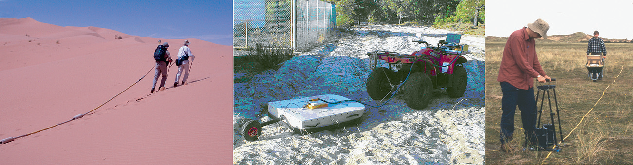
There are two common types of GPR which differ in the way that data are acquired, either in the time domain (impulse radar) or the frequency domain (continuous-wave and stepped- frequency radars). The resulting waveform indicates the amplitude of the energy scattered from subsurface objects in the time domain. The recorded signal is displayed in two-way traveltime (twt), the time taken for the pulse to travel down through the ground to the subsurface object and to return back to the surface where it is recorded. When selecting a radar system for a survey one critical choice is the antennas which come in a variety of shapes and sizes. First is the choice of antenna frequency which together with the velocity of the radar signal through the ground determines the wavelength of the signal, resolution, and depth of penetration. Lower-frequency antennas, for example, 10–50 MHz produce longer wavelength signals with lower resolution and increased depths of penetration; whereas higher- frequency antennas, for example, 200–500 MHz produce shorter wavelength signals with higher resolution but reduced depths of penetration. Having selected an appropriate wavelength for the objectives of the survey (see Jol and Bristow, 2003), there are different types of antennas available. There are at least four different types of antennas in common use: bistatic antennas, monostatic antennas, shielded/unshielded antennas, and rough terrain antennas (RTA) (Figure2).
Monostatic antennas have a single antenna that transmits and receives. Examples of unshielded bistatic antennas are shown in figure 2. There are two antennas which look like skis, one transmitting and the other receiving, which are moved across the ground at a constant separation in steps that can be determined by the user. Shielded antennas may be monostatic or bistatic and housed within a case which usually incorporates a Faraday cage or absorbing material that helps to reduce interference from external sources of EM radiation. The advantages are that the shielded antennas are generally more robust figure 2, and can be towed across the ground more easily than the unshielded ski type.
Stepped Frequency Continuous Wave (SFCW) radars have some advantages over the time domain GPRs: larger frequency bandwidth (Daniels, 1996; Taylor, 2001), higher mean power, lower noise figure, and, probably the most important one, the possibility of shaping the power spectral density. The last feature allows changing the level of the side lobes just by changing the “windowing” function. Of course, there is a price to be paid which regards the range resolution.
During this work we use the instrument SFCW GPR developed by the team of CNR Italy, (R.Persico) in the frequency range 50-1000MHz.
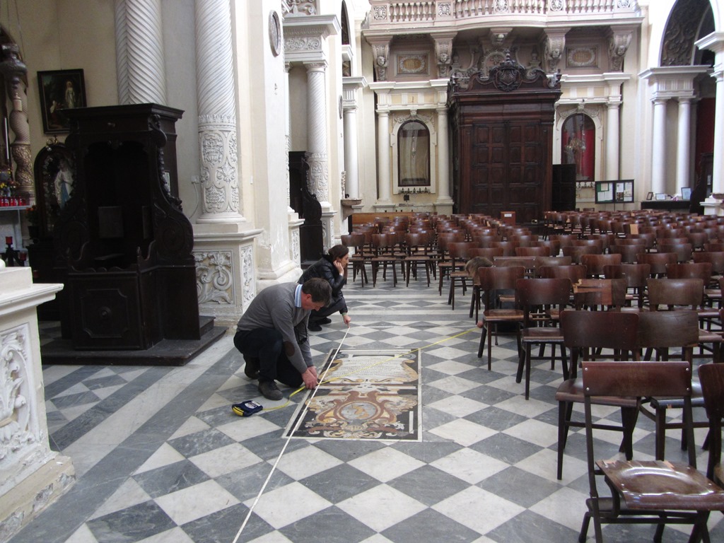
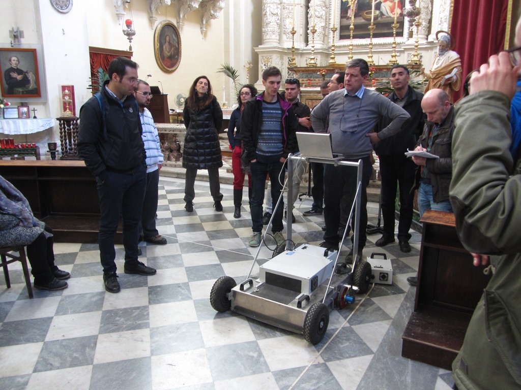
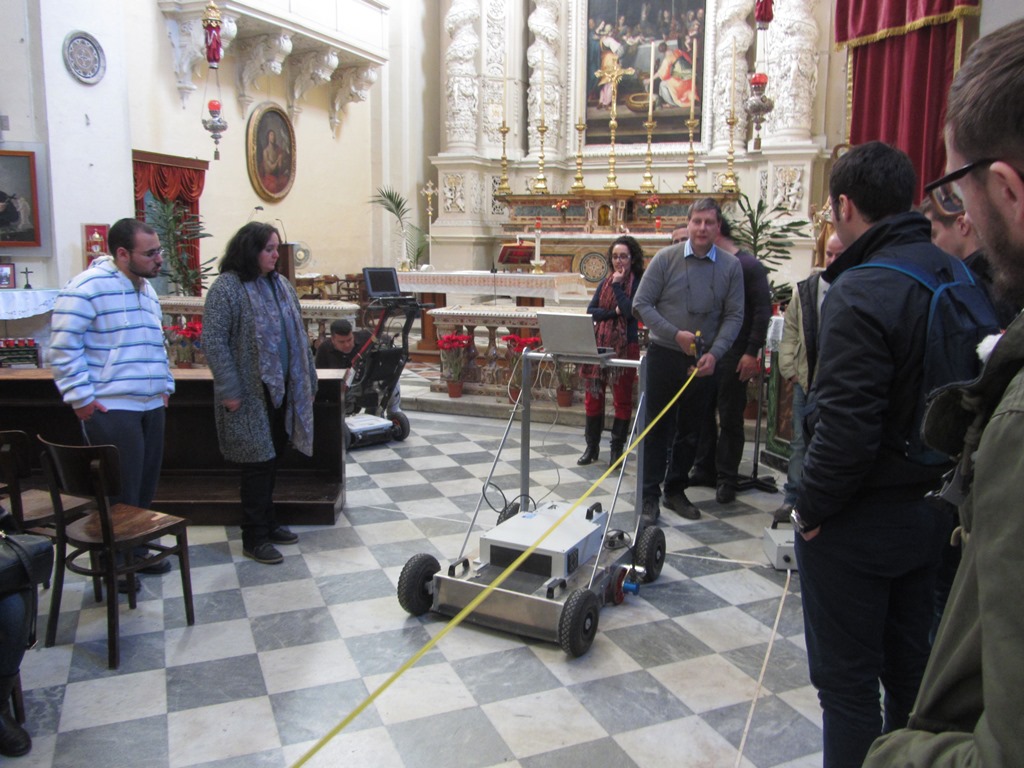
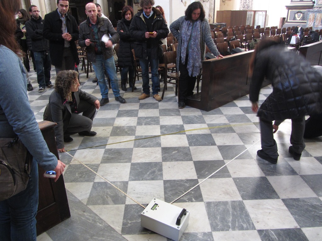
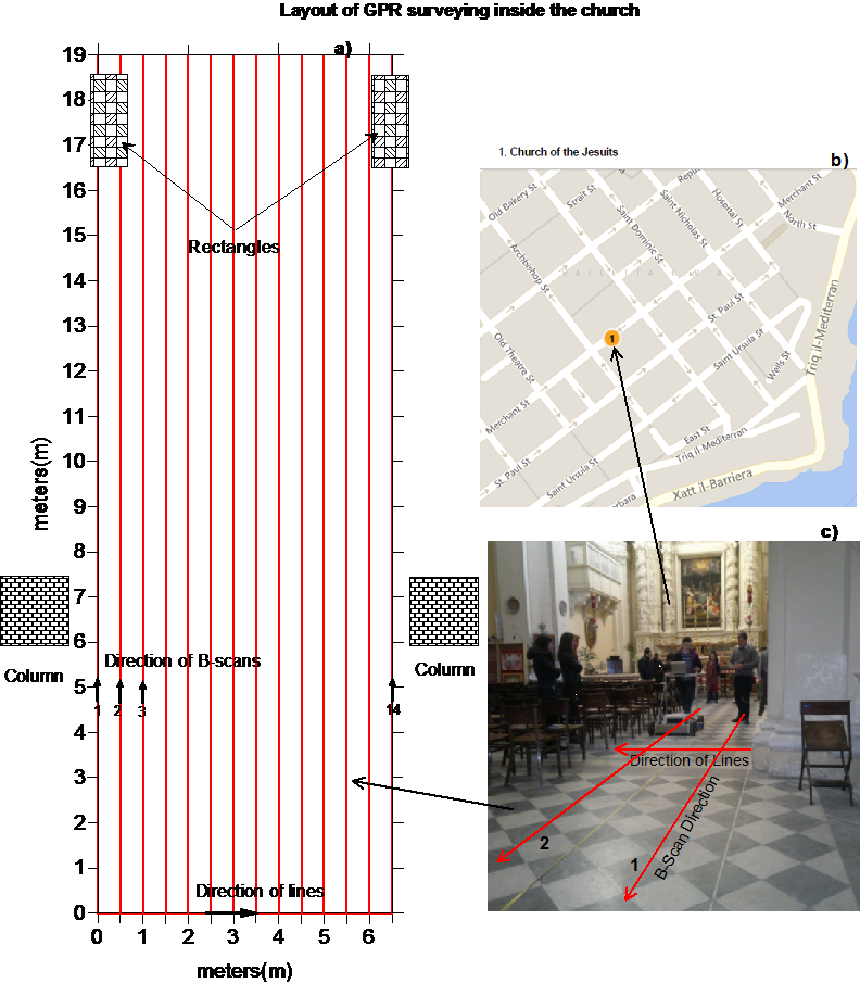
With this prototype instrument was surveyed the area in the basement of chapel with B-scans at distance intervals of 0.5m. The length of the B-scan lines was 19m. Notes related to possible object in basement were taken into account. The layout Grid of 3D GPR survey is shown in figure 7.
Processing, Imaging, and Inversion of GPR Data
Some form of signal processing will almost certainly have to be applied to GPR data and many functions can be performed during data processing (Figure 8). However, there is an old adage that should be remembered ‘rubbish in equals rubbish out.’ No amount of processing can compensate for poor data collection in the first place. If the data collected in the field is not good, all the processing in the world will not turn it into good data, and there is a lot to be said for the use of minimum processing in order to retain the integrity of the data. With this proviso in mind there are some basic processing steps that should be followed Cassidy (2009b) for further details. The first step is to edit the data files, removing bad traces or start positions if files need to be merged together to form longer lines. Dewow filters remove a low-frequency ‘wow’ and DC signal, reducing the data to a mean zero level. Dewow is generally an automatic function on most radar systems. Time-zero correction picks the first arrival of the direct air wave arrival at the receiver to correct for drift due to instability in the electronics or small changes in antenna configurations or air gaps where the antennas are not directly on the ground.
Filters can be applied that average down the trace (temporal) or from trace to trace (spatial) with the effect of smoothing the data and removing high-frequency noise. These filters should be used with discretion because excessive averaging between traces or down the trace will smooth the data. Additional high-pass filters allow the higher- frequency components to pass, removing low-frequency components. In contrast low-pass filters can be used to remove high-frequency noise while allowing the lower-frequency component to pass. High-pass and low-pass filters can be combined in band-pass filters that let through frequencies either side of the peak frequency of the transmitted radar signal. In order to convert the GPR profiles from the time domain in which the data are recorded to depth beneath the surface requires the velocity. Estimate of the average subsurface velocity can be extracted from ground truthing, collecting data above an object of known depth, or more commonly collection of CMP surveys. In addition, velocities can be estimated from matching modeled hyperbolic curves to diffractions or hyperbolas in the observed data. Field data will require static corrections for elevation changes along the profile. Topographic data should be collected in the field at the same time as the GPR profiles are collected using levels, laser levels, total stations, global positioning system (GPS) or differential global positioning system (DGPS) equipment. Gains are applied to the GPR data to enhance the appearance of later arrivals and compensate for the effects of signal attenuation and geometrical spreading loss.
There are a variety of gain functions but the most common are constant, spherical and exponential compensation (SEC) and automatic gain control (AGC). Migration to collapse hyperbolas and correct the position of dipping reflections is strongly recommended by Neal (2004) for GPR profiles in sediments but Cassidy (2009b) urges caution in applying migration because it can generate artifacts that could be misinterpreted. It is important to compare the profiles before and after each step in the processing to check that the profile is being enhanced by processing and to be aware that processing can generate artifacts.

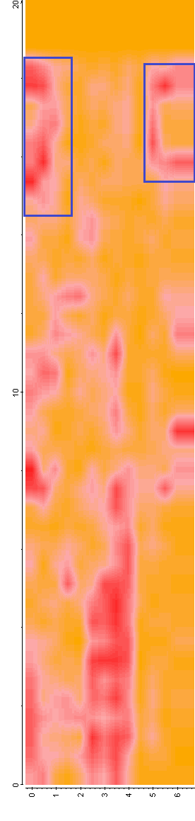
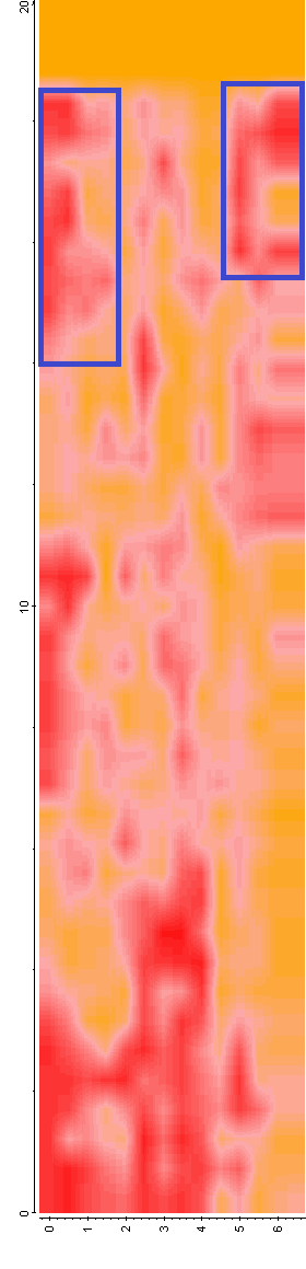
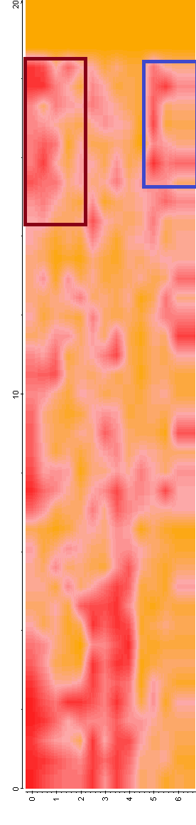
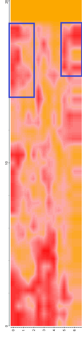
The GPR measurements on the Jeuist’s Church were collected in frequency domain. For each B-scan three measurements are collected in different frequencies (200, 400, 600 MHz). They are transformed in time domain and the general steps followed in the processing of raw data are: static muting correction (move start time); background removal (2D filter): Linear gain; 1D filter and migration in a propagation velocity of EM filed, of 0.09 m/s. The following filtering procedure was implemented in all the B-scans for the case of 400MHz antenna central frequency. A 3D interpretation of data is given in timeslices (horizontal sections) which represent the different depth of investigation.
From the time slices in different time, can be seen anomalies of strong reflections which could be related with underground buried structures (figure 9-12), such as: the foundations of columns and the rectangles may be related to buried stones. Strong reflection (red color) continues until a two way travel time below 30ns which corresponds with an approximately depth of 1.35m (velocity 0.09m/s), where are almost the anomalies detected on this place. Below this depth the reflections vanish and no anomalies are detected.
Conclusions
A multitude of existing and emerging GPR applications show the ability to non invasively image the subsurface with high resolution. Due to the rapidly evolving GPR surveying techniques, it is nowadays possible to acquire high-density, high-quality GPR data with high positioning accuracy. Most processing, imaging, and inversion tools are often based on approximations that include far-field, high-frequency raybased approximations, use a linearized system of equations, assume a two-dimensional space, or use only part of the data that enables a qualitative reconstruction of the subsurface properties.
Frequency Continuous Wave (SFCW) GPR have some advantages over the pulsed ones, because a range of frequencies is used (50-1000MHz). The timeslices show the case, were the medium frequency was chosen for B scans (400MHz). The main disadvantage is that more time is needed for processing the data. Data should be transformed in time domain for each B-scan and the processing steps have to be carried out in time domain. Several anomalies exist under the basement of Jesuit’s church, which could be related to stones and foundations of columns, which show strong reflection anomalies.
Acknowledgments: Authors thank the COST action for the financial support of this training school and the University of Malta for the valuable collaboration and hospitality.
References
Amir M. Alani , Morteza Aboutalebi, Gokhan Kilic (2013) Applications of ground penetrating radar (GPR) in bridge deck monitoring and assessment. Journal of Applied Geophysics 97 (2013) 45–54.
Annan AP (2002) GPR—History, trends and future developments. Subsurface Sensing Technologies and Applications 3: 253–270.
Annan AP (2005a) Ground-penetrating radar. In: Butler DK (ed.). Near Surface Geophysics, pp. 357–438. Tulsa, OK: SEG Press.
Benedetto, A., and Pajewski, L.,2015. Civil Engineering Applications of Ground Penetrating Radar. Springer Edition 2015, pp 3-39.
Binley A, Winship P, Middleton R, Pokar M, and West J (2001) High resolution characterization of vadose zone dynamics using cross-borehole radar. Water Resources Research 37: 2639–2652.
Blindow N (2006) Ground penetrating radar. In: Kirsch R (ed.) Groundwater Geophysics, pp. 357–438. Tulsa, OK: SEG Press.
Bristow, C.S., Jol, H.M. (Eds.), Ground Penetrating Radar in Sediments. The Geological Society, London, Special Publication 211. pp. 9–27.
Cassidy, N.J., 2009b. Ground-penetrating radar data processing, modeling and analysis. In: Jol, H.M. (Ed.), Ground Penetrating Radar: Theory and Applications. Elsevier, Amsterdam, pp. 141–176.
Cassidy, N.J., 2009b. Ground-penetrating radar data processing, modeling and analysis. In: Jol, H.M. (Ed.), Ground Penetrating Radar: Theory and Applications. Elsevier, Amsterdam, pp. 141–176.
Conyers LB and Goodman D (1997) Ground Penetrating Radar: An Introduction for Archaeologists. Walnut Creek, CA: AltaMira Press, 232 pp.
Daniels DJ (2004) Ground Penetrating Radar, 2nd edn. UK: Institution of Engineering and Technology.
Daniels, D.J., 1996. Surface Penetrating Radar. IEE Press.
Giovanni Alberti, Luca Ciofaniello, Marco Della Noce, Salvatore Esposito, Giovanni Galiero, Raffaele Persico, Marco Sacchettino and Sergio Vetrella, 2002, A stepped frequency GPR system for underground prospecting. ANNALS OF GEOPHYSICS, VOL. 45, N. 2, April 2002.
Hugenschmidt J (2002) Concrete bridge inspection with a mobile GPR system. Construction and Building Materials 16: 147–154.
Huisman JA, Hubbard SS, Redman JD, and Annan AP (2003) Measuring soil water content with ground penetrating radar: A review. Vadose Zone Journal 2: 476–491.
Huisman JA, Hubbard SS, Redman JD, and Annan AP (2003) Measuring soil water content with ground penetrating radar: A review. Vadose Zone Journal 2: 476–491.
Jadoon KZ, Weihermueller L, Scharnagl B, et al. (2012) Estimation of soil hydraulic parameters in the field by integrated hydrogeophysical inversion of time-lapse ground-penetrating radar data. Vadose Zone Journal 11. http://dx.doi.org/10.2136/vzj2011.0177.
Jol HM (2009) Ground Penetrating Radar Theory and Applications. Amsterdam: Elsevier Science.
Jol, H.M. (Ed.), 2009. Ground Penetrating Radar: Theory and Applications. Elsevier, Amsterdam, 524 p.
Jol, H.M., and Bristow, C.S., 2003. GPR in sediments: advise on data collection, basic processing and interpretation, a good practice guide. In: Bristow, C.S., Jol, H.M. (Eds.), Ground Penetrating Radar in Sediments. The Geological Society, London, Special Publication 211. pp. 9–27.
Jol, H.M., and Bristow, C.S., 2003. GPR in sediments: advise on data collection, basic processing and interpretation, a good practice guide. In:
Kalogeropoulos A, van der Kruk J, Hugenschmidt J, Busch S, and Merz K (2011) Chlorides and moisture assessment in concrete by GPR full waveform inversion. Near Surface Geophysics 9: 277–285.
Knight R (2001) Ground penetrating radar for environmental applications. Annual Review of Earth and Planetary Sciences 29: 229–255.
Lambot S, Slob EC, van den Bosch E, Stockbroeckx B, Scheers B, and Vanclooster M (2004) Estimating soil electric properties from monostatic ground-penetrating radar signal inversion in the frequency domain. Water Resources Research 40, W04205.
Lambot S, Weihermuller L, Huisman JA, et al. (2006) Analysis of air-launched ground penetrating radar techniques to measure the soil surface water content. Water Resources Research 42, W11403.
Redman JD, Davis JL, Galagedara LW, et al. (2002) Field studies of GPR air launched surface reflectivity measurements of soil water content. Proceedings of the Society of Photo-Optical Instrumentation Engineers (SPIE) 4758: 156–161.
Slob EC, Sato M, and Olhoeft G (2010) Surface and borehole ground-penetrating-radar developments. Geophysics 75: A103–A120.
Taylor, D., 2001. Ultra-wideband technology. CRC Press.
Van der Kruk, J., Tools and Techniques: Ground-Penetrating Radar, In Treatise on Geophysics (Second Edition) Editor-in-Chief: Gerald Schubert ISBN: 978-0-444-53803-1, Chapter 11.07, Pages 209-232
Weihermu¨ller L, Huisman JA, Lambot S, Herbst M, and Vereecken H (2007) Mapping the spatial variation of soil water content at the field scale with different ground penetrating radar techniques. Journal of Hydrology 340: 205–216.